
说明
本文是个人学习用的非官方中英对照译文,原文:https://diveintosystems.org/book/C7-x86_64/matrices.html。
原书采用 CC BY-NC-ND 4.0 许可(禁止演绎),请勿公开传播本译文。
标为「译注」「现代更新」的内容是译者补充,不代表原书作者观点;代码与原文逐字一致,未作改动。
7.8. Matrices
矩阵是一个二维数组。C 中的矩阵可以静态分配为二维数组(M[n][m]),可以通过一次 malloc 调用动态分配,也可以动态分配为一个「数组的数组」。我们来考虑数组的数组这种实现。第一个数组包含 n 个元素(M[n]),矩阵中的每个元素 M[i] 又包含一个由 m 个元素组成的数组。下面的代码片段各自声明了一个 4 × 3 的矩阵:
A matrix is a two-dimensional array. A matrix in C can be statically allocated as a two-dimensional array (
M[n][m]), dynamically allocated with a single call tomalloc, or dynamically allocated as an array of arrays. Let’s consider the array of arrays implementation. The first array containsnelements (M[n]), and each elementM[i]in our matrix contains an array ofmelements. The following code snippets each declare matrices of size 4 × 3:
1 | //statically allocated matrix (allocated on stack) |
在动态分配矩阵的情况下,主数组包含一个连续的 int 指针数组,每个整型指针指向内存中一个不同的数组。图 1 展示了我们通常如何直观地想象这两种矩阵。
In the case of the dynamically allocated matrix, the main array contains a contiguous array of
intpointers. Each integer pointer points to a different array in memory. Figure 1 illustrates how we would normally visualize each of these matrices.
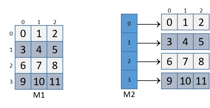
图 1. 静态分配(M1)和动态分配(M2)的 3x4 矩阵示意图
Figure 1. Illustration of a statically allocated (M1) and a dynamically allocated (M2) 3x4 matrix
对于这两种矩阵声明,都可以用双下标语法 M[i][j] 访问元素 (i,j),其中 M 是 M1 或 M2。不过,这两个矩阵在内存中的组织方式不同。尽管两者都把各自主数组中的元素连续存放在内存中,但我们的静态分配矩阵还把所有的行也连续存放在内存中,如图 2 所示。
For both of these matrix declarations, element (i,j) can be accessed using the double-indexing syntax
M[i][j], whereMis eitherM1orM2. However, these matrices are organized differently in memory. Even though both store the elements in their primary array contiguously in memory, our statically allocated matrix also stores all the rows contiguously in memory, as shown in Figure 2.

图 2. 矩阵 M1 按行主序的内存布局
Figure 2. Matrix M1’s memory layout in row-major order
对于 M2,并不能保证这种连续的排列。回想一下,要在堆上连续地分配一个 n × m 的矩阵,应当用一次 malloc 调用分配 n × m 个元素:
This contiguous ordering is not guaranteed for
M2. Recall that to contiguously allocate an n × m matrix on the heap, we should use a single call tomallocthat allocates n × m elements:
1 | //dynamic matrix (allocated on heap, memory efficient way) |
回想一下,对于 M3 这样的声明,不能用 M[i][j] 记法访问元素 (i,j),而必须用 M3[i*COLS + j] 的格式来索引元素。
Recall that with the declaration of
M3, element (i,j) cannot be accessed using theM[i][j]notation. Instead, we must index the element using the formatM3[i*COLS + j].
7.8.1. 连续的二维数组
7.8.1. Contiguous Two-Dimensional Arrays
考虑一个函数 sumMat,它的第一个参数是指向一个连续分配的(静态分配的或以节省内存的方式动态分配的)矩阵的指针,另外两个参数是行数和列数,它返回矩阵中所有元素的和。
Consider a function
sumMatthat takes a pointer to a contiguously allocated (either statically allocated or memory-efficiently dynamically allocated) matrix as its first parameter, along with the numbers of rows and columns, and returns the sum of all the elements inside the matrix.
在下面的代码片段中,我们使用按比例计算下标的方式,因为它同时适用于静态分配和动态分配的连续矩阵。回想一下,语法 m[i][j] 不适用于前面讨论的节省内存的连续动态分配。
We use scaled indexing in the code snippet that follows because it applies to both statically and dynamically allocated contiguous matrices. Recall that the syntax
m[i][j]does not work with the memory-efficient contiguous dynamic allocation previously discussed.
1 | int sumMat(int *m, int rows, int cols) { |
下面是对应的汇编,每一行都加上了英文注解:
Here is the corresponding assembly. Each line is annotated with its English translation:
1 | Dump of assembler code for function sumMat: |
局部变量 i、j 和 total 分别被加载到栈上的地址 %rbp-0xc、%rbp-0x8 和 %rbp-0x4 处。输入参数 m、row 和 cols 分别存放在位置 %rbp-0x8、%rbp-0x1c 和 %rbp-0x20 处。利用这些知识,我们把目光集中到只处理访问矩阵中元素 (i,j) 的那一部分:
The local variables
i,j, andtotalare loaded at addresses%rbp-0xc,%rbp-0x8, and%rbp-0x4on the stack, respectively. The input parametersm,row, andcolsare stored at locations%rbp-0x8,%rbp-0x1c, and%rbp-0x20, respectively. Using this knowledge, let’s zoom in on the component that just deals with the access of element (i,j) in our matrix:
译注
对照上面的汇编(mov %rdi,-0x18(%rbp)),参数 m 存放在 %rbp-0x18 而不是 %rbp-0x8(后者是 j),原文笔误。
1 | 0x4006ad <+39>: mov -0xc(%rbp),%eax # copy i to %eax |
第一组指令计算值 i*cols,并把它放在寄存器 %edx 中。回想一下,对于名为 matrix 的矩阵,matrix + (i * cols) 等价于 &matrix[i]。
The first set of instructions calculates the value
i*colsand places it in register%edx. Recall that for a matrix namedmatrix,matrix + (i * cols)is equivalent to&matrix[i].
1 | 0x4006b6 <+48>: mov -0x8(%rbp),%eax # copy j to %eax |
下一组指令计算 (i*cols+j)*4。编译器把下标 i*cols+j 乘以四,因为矩阵中的每个元素都是一个四字节的整数,这次乘法使编译器能算出正确的偏移量。<sumMat+53> 这一行的 cltq 指令是必需的,它把 %eax 的内容符号扩展为一个 64 位整数,因为这个值即将用于地址计算。
The next set of instructions computes
(i*cols+j)*4. The compiler multiplies the indexi*cols+jby four since each element in the matrix is a four-byte integer, and this multiplication enables the compiler to compute the correct offset. Thecltqinstruction on line<sumMat+53>is needed to sign-extend the contents of%eaxinto a 64-bit integer, since that is about to be used for address calculation.
接着,下面这组指令把算出的偏移量加到矩阵指针上,并对其解引用,得到元素 (i,j) 的值:
Next, the following set of instructions adds the calculated offset to the matrix pointer and dereferences it to yield the value of element (i,j):
1 | 0x4006c5 <+63>: mov -0x18(%rbp),%rax # copy m to %rax |
第一条指令把矩阵 m 的地址加载到寄存器 %rax。add 指令把 (i*cols + j)*4 加到 m 的地址上,正确地算出元素 (i,j) 的偏移位置。第三条指令对 %rax 中的地址解引用,并把值放到 %eax 中。注意这里用 %eax 作为目标组成部分寄存器;由于我们的矩阵中存放的是整数,而一个整数占四个字节,所以再次使用组成部分寄存器 %eax 而不是 %rax。
The first instruction loads the address of matrix
minto register%rax. Theaddinstruction adds(i*cols + j)*4to the address ofmto correctly calculate the offset of element (i,j). The third instruction dereferences the address in%raxand places the value in%eax. Notice the use of%eaxas the destination component register; since our matrix contains integers, and an integer takes up four bytes of space, component register%eaxis again used instead of%rax.
最后一条指令把 %eax 中的值加到累加器 total 上,它位于栈地址 %rbp-0x4 处。
The last instruction adds the value in
%eaxto the accumulatortotal, which is located at stack address%rbp-0x4.
我们来考虑如何访问图 2 中的元素 (1,2)。为方便起见,下面再列出这张图:
Let’s consider how element (1,2) is accessed in Figure 2. For convenience, the figure is reproduced below:
图 3. 矩阵 M1 按行主序的内存布局
Figure 3. Matrix M1’s memory layout in row-major order
元素 (1,2) 位于地址 M1 + 1*COLS + 2 处。由于 COLS = 3,元素 (1,2) 对应于 M1+5。要访问这个位置上的元素,编译器必须把 5 乘以 int 数据类型的大小(四个字节),得到偏移位置 M1+20,它对应于图中的字节 x20。对这个位置解引用,得到元素 5,它确实是矩阵中的元素 (1,2)。
Element (1,2) is located at address
M1 + 1*COLS + 2. SinceCOLS= 3, element (1,2) corresponds toM1+5. To access the element at this location, the compiler must multiply 5 by the size of theintdata type (four bytes), yielding the offsetM1+20, which corresponds to byte x20 in the figure. Dereferencing this location yields element 5, which is indeed element (1,2) in the matrix.
7.8.2. 不连续的矩阵
7.8.2. Noncontiguous Matrix
不连续的矩阵实现要稍微复杂一些。图 4 直观地展示了 M2 在内存中可能的布局。
The noncontiguous matrix implementation is a bit more complicated. Figure 4 visualizes how
M2may be laid out in memory.
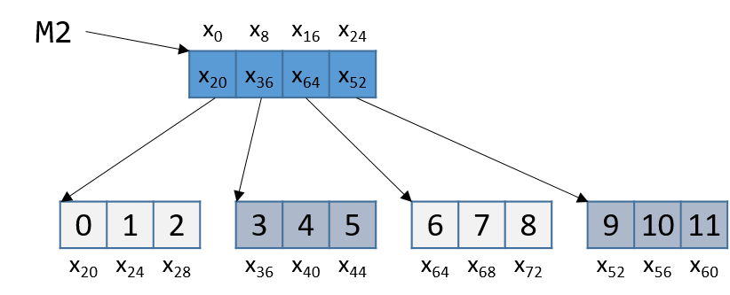
图 4. 矩阵 M2 在内存中的不连续布局
Figure 4. Matrix M2’s noncontiguous layout in memory
注意,指针数组是连续的,M2 的每个元素所指向的数组(例如 M2[i])也是连续的。然而,各个数组彼此之间并不连续。由于 M2 是一个指针数组,M2 的每个元素占八个字节。与之不同,由于 M2[i] 是一个 int 数组,M2[i] 的各个元素之间相距四个字节。
Notice that the array of pointers is contiguous, and that each array pointed to by an element of
M2(e.g.,M2[i]) is contiguous. However, the individual arrays are not contiguous with one another. SinceM2is an array of pointers, each element ofM2takes eight bytes of space. In contrast, asM2[i]is anintarray, each element ofM2[i]is four bytes away.
下例中的 sumMatrix 函数以一个整型指针数组(名为 matrix)作为第一个参数,以行数和列数作为第二个和第三个参数:
The
sumMatrixfunction in the following example takes an array of integer pointers (calledmatrix) as its first parameter, and a number of rows and columns as its second and third parameters:
1 | int sumMatrix(int **matrix, int rows, int cols) { |
尽管这个函数看起来与前面的 sumMat 函数几乎一模一样,但这个函数接收的矩阵由一个连续的指针数组构成。每个指针存放着一个单独的连续数组的地址,这个数组对应于矩阵中单独的一行。
Even though this function looks nearly identical to the
sumMatfunction shown earlier, the matrix accepted by this function consists of a contiguous array of pointers. Each pointer contains the address of a separate contiguous array, which corresponds to a separate row in the matrix.
下面是 sumMatrix 对应的汇编,每一行都加上了英文注解。
The corresponding assembly for
sumMatrixfollows. Each line is annotated with its English translation.
1 | Dump of assembler code for function sumMatrix: |
同样,变量 i、j 和 total 分别位于栈地址 %rbp-0xc、%rbp-0x8 和 %rbp-0x4 处。输入参数 matrix、row 和 cols 分别位于栈地址 %rbp-0x18、%rbp-0x1c 和 %rbp-0x20 处。我们把目光集中到专门处理访问元素 (i,j)(即 matrix[i][j])的那一部分:
Once again, the variables
i,j, andtotalare at stack addresses%rbp-0xc,%rbp-0x8, and%rbp-0x4, respectively. The input parametersmatrix,row, andcolsare located at stack addresses%rbp-0x18,%rbp-0x1c, and%rbp-0x20, respectively. Let’s zoom in on the section that deals specifically with an access to element (i,j), ormatrix[i][j]:
1 | 0x400715 <+39>: mov -0xc(%rbp),%eax # copy i to %eax |
这个例子中的五条指令计算 matrix[i],即 *(matrix+i)。由于 matrix[i] 中存放的是一个指针,i 首先被转换为 64 位整数。然后,编译器把 i 乘以八,再把它加到 matrix 上,以算出正确的地址偏移(回想一下,指针的大小是八个字节)。接着,<sumMatrix+59> 处的指令对算出的地址解引用,得到元素 matrix[i]。
The five instructions in this example compute
matrix[i], or*(matrix+i). Sincematrix[i]contains a pointer,iis first converted to a 64-bit integer. Then, the compiler multipliesiby eight prior to adding it tomatrixto calculate the correct address offset (recall that pointers are eight bytes in size). The instruction at<sumMatrix+59>then dereferences the calculated address to get the elementmatrix[i].
由于 matrix 是一个 int 指针数组,位于 matrix[i] 的元素本身就是一个 int 指针。matrix[i] 中的第 j 个元素位于 matrix[i] 数组中偏移 j × 4 处。
Since
matrixis an array ofintpointers, the element located atmatrix[i]is itself anintpointer. The jth element inmatrix[i]is located at offsetj × 4in thematrix[i]array.
下一组指令取出数组 matrix[i] 中的第 j 个元素:
The next set of instructions extract the jth element in array
matrix[i]:
1 | 0x40072c <+62>: mov -0x8(%rbp),%edx # copy j to %edx |
这段代码中的第一条指令把变量 j 加载到寄存器 %edx。<sumMatrix+65> 处的 movslq 指令把 %edx 转换为一个 64 位整数,把结果存放在 64 位寄存器 %rdx 中。接着,编译器用左移(shl)指令把 j 乘以四,并把结果存放在寄存器 %rdx 中。最后,编译器把得到的值加到 matrix[i] 中的地址上,得到元素 matrix[i][j] 的地址。<sumMatrix+75> 和 <sumMatrix+77> 处的指令取出 matrix[i][j] 处的值,并把它加到 total 上。
The first instruction in this snippet loads variable
jinto register%edx. Themovslqinstruction at<sumMatrix+65>converts%edxinto a 64-bit integer, storing the result in 64-bit register%rdx. The compiler then uses the left shift (shl) instruction to multiplyjby four and stores the result in register%rdx. The compiler finally adds the resulting value to the address located inmatrix[i]to get the address of elementmatrix[i][j]. The instructions at<sumMatrix+75>and<sumMatrix+77>obtain the value atmatrix[i][j]and add the value tototal.
我们回到图 4,考虑访问 M2[1][2] 的例子。为方便起见,下面再列出这张图:
Let’s revisit Figure 4 and consider an example access to M2[1][2]. For convenience, we reproduce the figure below:
图 5. 矩阵 M2 在内存中的不连续布局
Figure 5. Matrix M2’s noncontiguous layout in memory
注意,M2 从内存位置 x0 开始。编译器首先计算 M2[1] 的地址:把 1 乘以 8(sizeof(int *)),再加到 M2 的地址(x0)上,得到新地址 x8。对这个地址解引用,得到与 M2[1] 关联的地址,即 x36。然后,编译器把下标 2 乘以 4(sizeof(int)),并把结果(8)加到 x36 上,得到最终地址 x44。对地址 x44 解引用,得到值 5。果然,图 4 中对应于 M2[1][2] 的元素值为 5。
Note that
M2starts at memory location x0. The compiler first computes the address ofM2[1]by multiplying 1 by 8 (sizeof(int *)) and adding it to the address ofM2(x0), yielding the new address x8. A dereference of this address yields the address associated withM2[1], or x36. The compiler then multiplies index 2 by 4 (sizeof(int)), and adds the result (8) to x36, yielding a final address of x44. The address x44 is dereferenced, yielding the value 5. Sure enough, the element in Figure 4 that corresponds toM2[1][2]has the value 5.